
Ranger User Guide
- Table of Contents
- General System Info
- Environment
- Development
- Optimization
- Manuals & References
- General System Info
- Overview
- History
- System & Programming Notes
- Architecture
- System Access
- Environment
- Login Information
- Login Shell
- User Environment
- Startup Scripts
- Modules
- File Systems
- Login Information
- Development
- Programming Models
- Compilation
- Guidelines
- Serial
- Open MP
- MPI
- Basic Optimization
- Loading Libraries
- Running Code
- Runtime Environment
- Batch
- Interactive
- Process Affinity and Memory Policy
- Ranger Sockets
- Numactl
- Numa Control in Batch Scripts
- Tools
- Optimization
- General Optimization Guidelines
- Compiler Options
- Performance Libraries
- GotoBlas
- Code Tuning
- Manuals & References
Click on Header to expand or collapse section. PDF of General System Info section
Ranger is one of the largest computational resources in the world, serving NSF TeraGrid researchers throughout the United States, academic institutions within Texas, and the components of The University of Texas System.
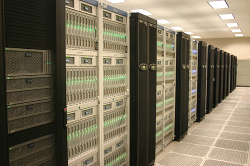
The Sun Constellation Linux Cluster, Ranger, is configured with 3,936 16-way SMP compute-nodes (blades), 123TB of total memory and 1.73PB of global disk space. The theoretical peak performance is 504 TFLOPS. Nodes are interconnected with InfiniBand technology in a full-CLOS topology providing a 1GB/sec point-to-point bandwidth. Also, a 2.8PB archive system and 5TB SAN network storage system are available through the login/development nodes.
 |
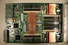 |
| Figure 2. SunBlade x6420 motherboard. | |
 |
|
| Figure 1. One of 6 rows:Management/IO Racks (black), Compute Rack (silver), and In-row Cooler (black). | Figure 3. Constellation Switch (partially wired). |
Project summary:
TACC and The University of Texas at Austin lead a project team that includes Sun Microsystems, Arizona State University, and Cornell University to build, deploy, operate, and support a new supercomputer of unprecedented capabilities under the National Science Foundation's HPC Systems Acquisitions program. The new system, Ranger, will be one of the more powerful supercomputing systems in the world when it enters full production in February 2008, offering 1/2 petaflop of performance, 1.7 petabytes of disk, and 125 terabytes of memory. Ranger will enable researchers to address problems that are too computationally demanding for today's terascale systems, stimulating and accelerating research across domains that advance science and society.
Configuration/Capabilities:
504 Teraflops of compute power, 3,936 Sun four-socket blades, 15,744 AMD " Barcelona" processors, Quad-core, four flops/cycle (dual pipelines), 125 Terabytes aggregate memory, 2 GB/core, 32 GB/node, 132 GB/s aggregate bandwidth, 1.7 Petabytes disk, 72 Sun x4500 aggregate "Thumper" I/O servers, 24TB each, 72 GB/sec total sec 1 PB in I/O bandwidth, largest filesystem, 10 Gbps / 2.3 latency Sun InfiniBand-based switches (2), up to 3456 4x ports each, Full non-blocking 7-stage Clos fabric.
Progress & Plans
Ranger is being constructed in TACC’s new machine room, located on the J.J. Pickle Research Campus in Austin, Texas. As of SC07, all compute, storage, and management hardware is in place, and cabling/integration and scalability testing is in progress. Ranger will be accessible to initial users in December 2007, and is scheduled for full production status as the TeraGrid’s most powerful resource in February 2008.
Photo Journal of the Ranger build
-

Empty machine room
Photographed by Kent Milfeld, December, 2006
-

Raised floor with chillers
Photographed by ? , March 6, 2007 -

Chiller racks
Photographed by Kent Milfeld, March 6, 2007 -

Power supply delivery
Photographed by Kent Milfeld, March 12, 2007 -

More power installed
Photographed by Kent Milfeld, March 12, 2007 -

One of many deliveries
Photographed by Kent Milfeld, March 21, 2007 -

Ranger nodes on dock
Photographed by Kent Milfeld, September 15, 2007 -

Many deliveries
Photographed Kent Milfeld, September 28, 2007 -

Magnum assembly
Photographed by Kent Milfeld, June 26, 2007 -

Magnum switch
Photographed by Kent Milfeld, October 26, 2007 -

Magnum switch
Photographed by Kent Milfeld, December 17, 2007 -

Ranger Blade
Photographed by Kent Milfeld, September 20, 2007 -

Ranger rack
Photographed by Kent Milfeld, October 26, 2007 -

Ranger row view
Photographed by Jo Wozniak, October 23, 2007 -

Ranger footprint
Photographed by Kent Milfeld, October 26, 2007
- Login Nodes now have barcelona chips
- The 4-socket Login3 and Login4 (ranger.tacc.utexas.edu) nodes have been populated with barcelona chips.
*** These are 2.2 GHz chips, the compute nodes run at 2.0 GHz. (Do not run codes on the login nodes.) - Compiling on Login Nodes
- When you login to ranger.tacc.utexas.edu you will be connected to either login3.ranger.tacc.utexas.edu or login4.ranger.tacc.utexas.edu (login1 and login2 are not available yet).
- MPI Support for Compilers
- Only the Intel and PGI compilers will support MPI. The mvapich2 libraries have been compiled with both compilers, and are automatically linked by the mpicc and mpif90 compiler drivers when correctly loaded throught the module commands. (By default the MPI compiler drivers use the PGI-compiled mvapich2 libraries and the default compilers are PGI.)
- Debugging and Profiling
- DDT is not available yet. Please use the idb (Intel) debugger, pgdbg and pgprof (PGI), and gdb and gprof (GNU) for debugging and profiling.
- /tmp on Compute Nodes
- In the compute nodes, the only physical storage device is an 8GB compact flash, which stores the OS. Only 150MB are available in /tmp for user storage. Program developers should use $SCRATCH to store temporary files. (The /tmp directories on login nodes are 36G disk devices.)
- Parallel Environment (using less than 16 cores/node)
- The Parallel Environment Section shows how to use less than 16 tasks per node, and how to run hybrid codes.
- MPI (mvapich) Options for Scalable code
- See the mvapich1/2 User Guides.
- Core Affinity and Memory Allocation Policy
- See Numa Section for controlling process/thread execution on sockets and cores; and memory allocation policy on sockets.
- Core Count for Batch SGE Jobs
- See Numa Section (look for MY_NSLOTS) for core counts other than a multiple of 16.
- Experienced Users
- Check out the Quick Start Notes.
The Ranger compute and login nodes run a Linux OS and are managed by the Rocks 4.1 cluster toolkit. Two 3456 port Constellation switches provide dual-plane access between NEMs (Network Element Modules) of each 12-blade chassis. Several global, parallel Lustre file sytems have been configured to target different storage needs. Each compute node contains 16 cores as a 4-socket, quad-core platform. The configuration and features for the compute nodes, interconnect and I/O systems are described below, and summarized in Tables 1-3.
- Compute Nodes: Ranger is a blade-based system. Each node is a SunBlade x6420 blade running a 2.2 x86_64 Linux kernel from kernel.org. Each node contains four AMD Opteron Quad-Core 64-bit processors (16 cores in all) on a single board, as an SMP unit. The core frequency is 2.0GHz and supports 4 floating-point operations per clock period with a peak performance of 8 GFLOPS/core or 128 GFLOPS/node.
Each node contains 32GB of memory. The memory subsystem has an 800MHz Hypertransport system Bus, and 2 channels with 667MHz Fully Buffered DIMMS. Each socket possesses an independent memory controller connected directly to L3 cache.
- Interconnect: The interconnect topology is a full-CLOS fat tree. Each of the 328 12-node compute chassis is connected directly to the 2 core switches. 12 additional frames are also connected directly to the core switches and provide files systems, administration and login capabilities.
- File systems: Ranger's file systems are built on 72 Sun x4500 disk servers, each containing 48 SATA drives, and two Sun x4600 metadata servers. From this aggregate space of 1.73PB, several file systems will be partitioned (see Table 5).
| Table 1. System Configuration & Performance | ||
| Component | Technology | Performance/Size |
| Peak Floating Point Operations |
504 TFLOPS (Theoretical) | |
| Nodes(blades) | Four Quad-Core AMD Opteron processors | 3,936 Nodes / 62,976 Cores |
| Memory | Distributed | 123TB (Aggregate) |
| Shared Disk | Lustre, parallel File System | 1.73PB |
| Local Disk | Compact Flash | 31.4TB (Aggregate) |
| Interconnect | InfiniBand Switch | 1 GB/s P-2-P Bandwidth |
| Table 2. SunBlade x6420 Compute Node | |
| Component | Technology |
| Sockets per Node/Cores per Socket | 4/4 (Barcelona) |
| Clock Speed | 2.0GHz |
| Memory Per Node | 32GB memory |
| System Bus | HyperTransport, 6.4GB bidirectional |
| Memory | 2GB DDR2/667, PC2-5300 ECC-registered DIMMs |
| PCI Express | x8 |
| Compact Flash | 8GB |
| Table 3. Sun x4600 Login Nodes | |
| Component | Technology |
| 4 login nodes |
ranger.tacc.utexas.edu (login1.tacc.utexas.edu Not Available) (login2.tacc.utexas.edu Not Available) (login3.tacc.utexas.edu) (login4.tacc.utexas.edu) |
| Sockets per Node/Cores per Socket | 4/4 (Barcelona). |
| Clock Speed | 2.2GHz |
| Memory Per Node | 32GB |
| Table 4. AMD Barcelona Processor | |
| Technology | 64-bit |
| Clock Speed | 2.0GHz |
| FP Results/Clock Period | 4 |
| Peak Performance/core | 8GFLOPS/core |
| L3 Cache | 2MB on-die (shared) |
| L2 Cache | 4 x 512KB |
| L1 Cache | 64KB |
| Table 5. Storage Systems | |||
| Storage Class | Size | Architecture | Features |
| Local | 8GB/node | Compact Flash | not available to users (O/S only) |
| Parallel | 1.73PB | Lustre, Sun x4500 disk servers | 72 Sun x4500 I/O data servers, 2 Sun x4600 Metadata servers (See Table 6 for breakdown of the parallel filesystems) |
| SAN | 15TB | Synergy FS, SUN Storage Tek | QLogic switch, SUN V880 Server, mnt on /san/hpc/<project> |
| Ranch (Tape Storage) | 2.8PB | SAMFS (Storage Archive Manager) | 10Gb/s connection through 8 GridFTP Servers |
| Table 6. Parallel Filesystems | |||
| Storage Class | Size | Quota (per User) | Features |
| HOME | ~100TB | 6GB | Backed up nightly; Not purged |
| WORK | ~200TB | 350GB | Not backed up; Not purged |
| SCRATCH | ~800TB | 400TB | Not backed up; Purged every 10 days |
SSH
To ensure a secure login session, users must connect to machines using the secure shell, ssh program. Telnet is no longer allowed because of the security vulnerabilities associated with it. The "r" commands rlogin, rsh, and rcp, as well as ftp, are also disabled on this machine for similar reasons. These commands are replaced by the more secure alternatives included in SSH --- ssh, scp, and sftp.
Before any login sessions can be initiated using ssh, a working SSH client needs to be present in the local machine. Go to the TACC introduction to SSH for information on downloading and installing SSH.
To initiate an ssh connection to a ranger login node, execute the following command on your local workstation
Note <login-name> is needed only if the user name on the local machine and the TACC machine differ.
ssh <login-name> @ ranger.tacc.utexas.edu
Additionally, each of the login nodes can be accessed directly, to allow users to move data to/from local disk space on the login nodes. These nodes are directly accessible by using the node name:
ssh <login-name> @ <login{3|4}>.ranger.tacc.utexas.edu
Password changes (with the passwd command) are forced to adhere to "strength checking" rules, and users are asked to comply with practices presented in the TACC password guide.
Click on Header to expand or collapse section. PDF of Environment section
Login Shell
The most important component of a user's environment is the login shell that interprets text on each interactive command line and statements in shell scripts. Each login has a line entry in the /etc/passwd file, and the last field contains the shell launched at login. To determine your login shell, execute:
| echo $SHELL | {to see your login shell} |
You can use the chsh command to change your login shell; instructions are in the man page. Available shells are listed in the /etc/shells file with their full-path. To change your login shell, execute:
| cat /etc/shells | {select a <shell> from list} |
| chsh -s <shell> <username> | {use full path of the shell} |
User Environment
The next most important component of a user's environment is the set of environment variables. Many of the Unix commands and tools, such as the compilers, debuggers, profilers, editors, and just about all applications that have GUIs (Graphical User Interfaces), look in the environment for variables that specify information they may need to access. To see the variables in your environment execute the command:
The variables are listed as keyword/value pairs separated by an equal (=) sign, as illustrated below by the HOME and PATH variables.
| HOME=/home/utexas/staff/milfeld |
| PATH=/bin:/usr/bin:/usr/local/apps:/opt/intel/bin |
(PATH has a colon (:) separated list of paths for its value.) It is important to realize that variables set in the environment (with setenv for C shells and export for Bourne shells) are "carried" to the environment of shell scripts and new shell invocations, while normal "shell" variables (created with the set command) are useful only in the present shell. Only environment variables are seen in the env (or printenv) command; execute set to see the (normal) shell variables.
Startup Scripts
All Unix systems set up a default environment and provide administrators and users with the ability to execute additional Unix commands to alter the environment. These commands are "sourced"; that is, they are executed by your login shell, and the variables (both normal and environmental) as well as aliases and functions are included in the present environment. We recommend that you customize the login environment by inserting your "startup" commands in .cshrc_user, .login_user, and .profile_user files in your home directory.
Basic site environment variables and aliases are set in
| /usr/local/etc/cshrc | {C-shell, non-login specific} |
| /usr/local/etc/login | {C-shell, specific to login} |
| /usr/local/etc/profile | {Bourne-type shells} |
For historical reasons, the C shells source two types of files. The .cshrc type files are sourced first (/etc/csh.cshrc--> $HOME/.cshrc--> /usr/local/etc/cshrc--> $HOME/.cshrc_user). These files are used to set up environments that are to be executed by all scripts and used for access to the machine without a login. For example, the following commands only execute the .cshrc type files on the remote machine:
| scp data ranger.tacc.utexas.edu: | {only .cshrc sourced on ranger} |
| ssh ranger.tacc.utexas.edu date | {only .cshrc sourced on ranger} |
The .login type files are used to setup environment variables that you commonly use in an interactive session. They are sourced after the .cshrc type files (/etc/csh.login--> $HOME/.login--> /usr/local/etc/login-->
$HOME/.login_user). Similarly, if your login shell is a Bourne shell (bash, sh, ksh, ...), the profile files are sourced (/etc/profile--> $HOME/.profile--> /usr/local/etc/profile--> $HOME/.profile_user).
The commands in the /etc files above are concerned with operating system behavior and set the initial PATH, ulimit, umask, and environment variables such as the HOSTNAME. They also source command scripts in /etc/profile.d -- the /etc/csh.cshrc sources files ending in .csh, and /etc/profile sources files ending in .sh. Many site administrators use these scripts to setup the environments for common user tools (vim, less, etc.) and system utilities (ganglia, modules, Globus, LSF, etc.)
TACC has to coordinate the environments on platforms of several operating systems: AIX, Linux, IRIX, Solaris, and Unicos. In order to efficiently maintain and create a common environment among these systems, TACC uses its own startup files in /usr/local/etc. (A corresponding file in this etc directory is sourced by the .profile, , and .login files that reside in your home directory. (Please do not remove these files and the sourcing commands in them, even if you are a Unix guru.) Any commands that you put in your .login_user, .cshrc_user, or .profile_user file are sourced (if the file exists) at the end of the corresponding /usr/local/etc command files. If you accidentally remove your .login, .cshrc, and .login, you can copy new ones from /usr/local/etc/start-up or execute
to get a new copy (your old files are renamed with a date suffix).
Modules
TACC is constantly including updates and installing revisions for application packages, compilers, communications libraries, and tools and math libraries. To facilitate the task of updating and to provide a uniform mechanism for accessing different revisions of software, TACC uses the modules utility.
At login, a basic environment for the default compilers, tools, and libraries is set by several modules commands. Your PATH, MANPATH, LIBPATH, directory locations (WORK, HOME, ...), aliases (cdw ...) and license paths, are just a few of the environment variables and aliases created for you. This frees you from having to initially set them and update them whenever modifications and updates are made in system and application software.
Users who need 3rd party applications, special libraries, and tools for their development can quickly tailor their environment with only the applications and tools they need. (Building your own specific application environment through modules allows you to keep your environment free from the clutter of all the other application environments you don't need.)
Each of the major TACC applications has a modulefile that sets, unsets, appends to, or prepends to environment variables such as $PATH, $LD_LIBRARY_PATH, $INCLUDE_PATH, $MANPATH for the specific application. Each modulefile also sets functions or aliases for use with the application. A user need only invoke a single command,
at each login to configure an application/programming environment properly. If you often need an application environment, place the modules command in your .login_user and/or .profile_user shell startup file.
Most of the package directories are in /opt/apps ($APPS) and are named after the package name (<app>). In each package directory there are subdirectories that contain the specific versions of the package.
As an example, the fftw package requires several environment variables that point to its home, libraries, include files, and documentation. These can be set in your environment by loading the fftw module:
To see a list of available modules and a synopsis of a modulefile's operations, execute:
| module available | {lists modules} |
| module help <app> | {lists environment changes performed for <app>} |
During upgrades, new modulefiles are created to reflect the changes made to the environment variables. TACC will always announce upgrades and module changes in advance.
The TACC HPC platforms have several different file systems with distinct storage characteristics. There are predefined, user-owned directories in these file systems for users to store their data. Of course, these file systems are shared with other users, so they are managed by either a quota limit, a purge policy (time-residency) limit, or a migration policy.
Three Lustre file systems are available to users: $HOME, $WORK and $SCRATCH. Users have 6GB for $HOME. $WORK on our Ranger system is NOT a purged file system, but is limited by a large quota. Use $SCRATCH for temporary, large file storage; this file sytem is purged periodically (TBD), and has a very large quota. All file systems also impose an inode limit.
To determine the size of a file system, cd to the directory of interest and execute the "df -k ." command.
Without the "dot" all file systems are reported. In the df command output below, the file system name appears on the left (IP number, "ib" protocol, using OFED gen2) , and the used and available space (-k, in units of 1KBytes) appear in the middle columns followed by the percent used and the mount point:
% df -k . File System 1k-blocks Used Available Use% Mounted on 129.114.97.1@o2ib:/share 103836108384 290290196 103545814376 1% /share
To determine the amount of space occupied in a user-owned directory, cd to the directory and execute the du command with the -sb option (s=summary, b=units in bytes):
du -sb
To determine quota limits and usage, execute the lfs quota command with your username and the directory of interest:
lfs quota -u <username> $HOME
lfs quota -u <username> $WORK
lfs quota -u <username> $SCRATCH
The four major file systems available on Ranger are:
- home directory
- At login, the system automatically changes to your home directory.
This is the recommended location to store your source codes and build your executables.
The quota limit on home is 6GB.
A user's home directory is accessible from the frontend node and any compute node.
Use $HOME to reference your home directory in scripts.
Use cd to change to $HOME. - work directory
- Store large files here.
Often users change to this directory in their batch scripts and run their jobs in this file system.
A user's work directory is accessible from the frontend node and any compute node.
The user quota is 350GB for Early Users, and will be set to a smaller value when $SCRATCH comes on line.
Purge Policy: There is no purging on this file system.
This file system is not backed up.
Use $WORK to reference your work directory in scripts.
Use cdw to change to $WORK. - scratch or temporary directory
- This file system is not on line yet.
- UNLIKE the TACC Lonestar system, this is NOT a local disk file system on each node.
This is a global Lustre file system for storing temporary files.
Purge Policy: Files on this system are purged when a file's access time exceeds 10 days.
PLEASE NOTE: TACC staff may delete files from scratch if the scratch file system becomes full and directories consume an inordinately large amount of disk space, even if files are less than 10 days old. A full file system inhibits use of the file system for all users. The use of programs or scripts to actively circumvent the file purge policy will not be tolerated.
Often, in batch jobs it is more efficient to use and store files directly in $WORK (to avoid moving files from scratch later before they are purged).
The quota on this system is 400TB.
Use $SCRATCH to reference this file system in scripts.
Use cds to change to $SCRATCH. - archive
More on Archive -- rls and sync not available yet
Click on Header to expand or collapse section. PDF of Development section
There are two distinct memory models for computing: distributed-memory and shared-memory. In the former, the message passing interface (MPI) is employed in programs to communicate between processors that use their own memory address space. In the latter, open multiprocessing (OMP) programming techniques are employed for multiple threads (light weight processes) to access memory in a common address space.
For distributed memory systems, single-program multiple-data (SPMD) and multiple-program multiple-data (MPMD) programming paradigms are used. In the SPMD paradigm, each processor loads the same program image and executes and operates on data in its own address space (different data). This is illustrated in Figure 4. It is the usual mechanism for MPI code: a single executable (a.out in the figure) is available on each node (through a globally accessible file system such as $WORK or $HOME), and launched on each node (through the batch MPI launch command, "ibrun a.out").
In the MPMD paradigm, each processor loads up and executes a different program image and operates on different data sets, as illustrated in Figure 4. This paradigm is often used by researchers who are investigating the parameter space (parameter sweeps) of certain models, and need to launch 10s or 100s of single processor executions on different data. (This is a special case of MPMD in which the same executable is used, and there is NO MPI communication.) The executables are launched through the same mechanism as SPMD jobs, but a Unix script is used to assign input parameters for the execution command (through the batch MPI launcher, "ibrun script_command"). Details of the batch mechanism for parameter sweeps are described in the Running Programs section.
 |
The shared-memory programming model is used on Symmetric Multi- Processor (SMP) nodes, like the TACC Champion Power5 System (8 CPUs, 16GB memory per node) or the TACC Ranger Cluster (16 cores, 32GB memory per node).
The programming paradigm for this memory model is called Parallel Vector Processing (PVP) or Shared-Memory Parallel Programming (SMPP). The latter name is derived from the fact that vectorizable loops are often employed as the primary structure for parallelization. The main point of SMPP computing is that all of the processors in the same node share data in a single memory subsystem, as shown in Figure 5. There is no need for explicit messaging between processors as with with MPI coding.
 |
In the SMPP paradigm either compiler directives (as pragmas in C, and special comments in FORTRAN) or explicit threading calls (e.g. with Pthreads) is employed. The majority of science codes now use OpenMP directives that are understood by most vendor compilers, as well as the GNU compilers.
In cluster systems that have SMP nodes and a high speed interconnect between them, programmers often treat all CPUs within the cluster as having their own local memory. On a node an MPI executable is launched on each CPU and runs within a separate address space. In this way, all CPUs appear as a set of distributed memory machines, even though each node has CPUs that share a single memory subsystem.
In clusters with SMPs, hybrid programming is sometimes employed to take advantage of higher performance at the node-level for certain algorithms that use SMPP (OMP) parallel coding techniques. In hybrid programming, OMP code is executed on the node as a single process with multiple threads (or an OMP library routine is called), while MPI programming is used at the cluster-level for exchanging data between the distributed memories of the nodes.
For further information on OpenMP, MPI and on programming models/paradigms, please see the manuals and packages sections of this document.
Compiler Usage Guidelines
The AMD Compiler Usage Guidelines document provides the "best-known" peak switches for various compilers tailored to their Opteron products. Developers and installers should read Chapter 5 of this document before experimenting with PGI and Intel compiler options.
See Chapter 5 of the AMD Compiler Usage Guidelines.
The Intel 10.1 Compiler Suite
The Intel 10.1 compilers are NOT the default compilers. You must use the module commands to load the Intel compiler environment (see above). (The 9.1 compilers are available for special porting needs.) The gcc 3.4.6 compiler and module are also available.We recommend using the Intel (or the PGI) suite whenever possible. The 10.1 suite is installed with the 64-bit standard libraries and will compile programs as 64-bit applications (as the default compiler mode).
Web accessible Intel manuals are available: Intel 10.1 C++ Compiler Documentation and Intel 10.1 Fortran Compiler Documentation.
The PGI 7.1 Compiler Suite
The PGI 7.1 compilers are loaded as the default compilers at login with the pgi module. We are recommending the use of the PGI suite whenever possible (at this time). The 7.1 suite is installed with the 64-bit standard libraries and will compile programs as 64-bit applications (as the default compiler mode).
A PDF version of the PGI User's Guide is avaiable.
Initially the Ranger programming environment will support several compilers: Intel, PGI, gcc and SUN. The first section explains how to use modules to set up the compiler environment. The next section presents the compiler invocation for serial and MPI executions, and follows with a section on options. All compiler commands can be used for just compiling with the -c option (create just the ".o" object files) or compiling and linking (to create executables).
By default, the pgi compiler environment is set up at login. To use a different compiler you must use module commands to first unload the MPI environment (mvapich2), swap the compiler environment, and then reload the MPI environment. Execute the module avail to determine the modulefile names for all the available compilers; they have the syntax compiler/version. The commands are listed below. Place these commands in your .login (C shells) or .profile (Bourne shells) file to automatically set an alternate default compiler in your environment at login.
module unload mvapich2 module swap pgi intel module load mvapich2
The compiler invocation commands for the supported vendor compiler systems are tabulated below.
Compiling Serial Programs
| Vendor | Compiler | Program | TypeSuffix |
| intel | icc | C | .c |
| intel | icc | C++ | .C, .cc, .cpp, .cxx |
| intel | ifort | F90 | .f, .for, .ftn, .f90, .fpp |
| pgi | pgcc | C | .c |
| pgi | pgcpp | C++ | .C, .cc |
| pgi | pgf95 | F77/90/95 | .f, .F, .FOR, .f90, .f95, .hpf |
| gnu | gcc | C | .c |
| sun | sun_cc | C | .c |
| sun | sun_CC | C++ | .C, .cc, .cpp, .cxx |
| sun | sunf90 | F77/90 | .f, .F, .FOR, .f90, .hpf |
| sun | sunf95 | F95 | .f, .F, .FOR, .f90, .f95, .hpf |
Appropriate program-name suffixes are required for each compiler. By default, the executable name is a.out. It may be renamed with the -o option. To compile without the link step, use the -c option. The following examples illustrate renaming an executable and the use of two important compiler optimization options:
intel icc/ifort -o flamec.exe -O2 -xW prog.c/cc/f90 pgi pgcc/pgcpp/pgf95 -o flamef.exe -fast -tp barcelona-64 prog.c/cc/f90 gnu gcc -o flamef.exe -mtune=barcelona -march=barcelona prog.c sun sun_cc/sun_CC/sunf90 -o flamef.exe -xarch=sse2 prog.c/cc/f90
A list of all compiler options, their syntax, and a terse explanation, is given when the compiler command is executed with the -help option. Also, man pages are available. To see the help or and man information, execute one of:
compiler -help / man compiler with compiler = ifort, pgf90/95 or sunf90 or gcc --help / man gcc
Some of the more important options are listed below.
Compiling Parallel Programs with MPI
The "mpicmds" commands support the compilation and execution of parallel MPI programs for specific interconnects and compilers. At login, MPI MVAPICH (mvapich2) and Intel 10.1 compiler (intel) modules are loaded to produce the default environment which provide the location to the corresponding mpicmds. Compiler scripts (wrappers) compile MPI code and automatically link startup and message passing libraries into the executable. Note that the compiler and MVAPICH library are selected according to the modules that have been loaded. The following table lists the compiler wrappers for each language:
Compiling Parallel Programs with MPI
Compiler Program TypeSuffix mpicc c .c mpiCC C++ .cc, .C, .cpp, .cxx mpif90 F77/F90 .f, .for, .ftn, .f90, .f95, .fpp
Appropriate program-name suffixes are required for each wrapper. By default, the executable name is a.out. It may be renamed with the -o option. To compile without the link step, use the -c option. The following examples illustrate renaming an executable and the use of two important compiler optimization options:
intel mpicc/mpif90 -o prog.exe -O2 -xW prog.cc/f90 pgi mpicc/mpif90 -o prog.exe -fast -tp barcelona-64 prog.f90
Include linker options such as library paths and library names after the program module names, as explained in the Loading Libraries section below. The Running Code section explains how to execute MPI executables in batch scripts and "interactive batch" runs on compute nodes.
We recommend that you use either the Intel or the PGI compiler for optimal code performance. TACC does not support the use of the gcc compiler for production codes on the Ranger system. For those rare cases when gcc is required, for either a module or the main program, you can specify the gcc compiler with the -cc mpcc option. (Since gcc- and Intel-compiled code are binary compatible, you should compile all other modules that don't require gcc with the Intel compiler.) When gcc is used to compile the main program, an additional Intel library is required. The examples below show how to invoke the gcc compiler in combination with the Intel compiler for the two cases:
mpicc -O2 -xW -c -cc=gcc suba.c
mpicc -O2 -xW mymain.c suba.o
mpicc -O2 -xW -c suba.c
mpicc -O2 -xW -cc=gcc -L$ICC_LIB -lirc mymain.c suba.o
Compiling OpenMP Programs
Since each of the blades (nodes) of the Ranger cluster is an AMD Opteron quad-processor quad-core system, applications can use the shared memory programming paradigm "on node". With a total number of 16 cores per node, we encourage the use of a shared-memory model on the node.
The OpenMP compiler options are listed below for those who do need SMP support on the nodes. For hybrid programming, use the mpi-compiler commands, and include the openmp options.
Intel : mpicc/mpif90 -O2 -xW -openmp
pgi : mpicc/mpif90 -fast -tp barcelona-64 -mp
Basic Optimization for Serial and Parallel Programming using OpenMP and MPI
The MPI compiler wrappers use the same compilers that are invoked for serial code compilation. So, any of the compiler flags used with the icc command can also be used with mpicc; likewise for ifort and mpif90; and iCC and mpiCC. Below are some of the common serial compiler options with descriptions.
Intel Compiler
Compiler Options Description -03 performs some compile time and memory intensive optimizations in addition to those executed with -O2, but may not improve performance for all programs. -ipo Interprocedural optimizations ‑vec_report[0|...|5] control amount of vectorizer diagnostic information: -xW includes specialized code for SSE and SSE2 instructions (recommended). -xO includes specialized code for SSE, SSE2 and SSE3 instructions. Use, if code benefits from SSE3 instructions. -fast -ipo, -O2, -static DO NOT USE -- static load not allowed. -g -fp debugging information produced, disable using EBP as general purpose register -openmp enable the parallelizer to generate multi-threaded code based on the OpenMP directives ‑openmp_report[0|1|2] control the OpenMP parallelizer diagnostic level. ‑help lists options
Developers often experiment with the following options: -pad, -align, -ip, -no-rec-div and -no-rec-sqrt. In some codes performance may decrease. Please see the Intel compiler manual (below) for a full description of each option.
Use the -help option with the mpicmds commands for additional information:
mpicc -help mpif90 -help mpirun -help {use the listed options with the ibrun cmd}
pgi Compiler
For detail on the MPI standard go to the URL: www.mcs.anl.gov/mpi.
Compiler Options Description -03 performs some compile time and memory intensive optimizations in addition to those executed with -O2, but may not improve performance for all programs. -Mipa=fast, inline Interprocedural optimizations There is a loader problem with this option. -tp barcelona-64 includes specialized code for the barcelona chip. -fast -O2 -Munroll=c:1 -Mnoframe -Mlre -Mautoinline -Mvect=sse -Mscalarsse -Mcache_align -Mflushz -g, -gopt debugging information produced -mp enable the parallelizer to generate multi-threaded code based on the OpenMP directives ‑Minfo=mp,ipa Information about OpenMP, interprocedural optimization ‑help lists options ‑help ‑fast lists options for -fast
Loading Libraries
Some of the more useful load flags/options are listed below. For a more comprehensive list, consult the ld man page.
- Use the -l loader option to link in a library at load time: e.g.
compiler prog.f90 -lname This links in either the shared library libname.so (default) or the static library libname.a, provided that the correct path can be found in ldd's library search path or the LD_LIBRARY_PATH environment variable paths.
- To explicitly include a library directory, use the -L option, e.g.
compiler prog.f -L/mydirectory/lib -lname In the above example, the user's libname.a library is not in the default search path, so the "-L" option is specified to point to the libname.a directory.
Many of the modules for applications and libraries, such as the mkl library module provide environment variables for compiling and linking commands. Execute module help module_name for a description, listing and use cases for the assigned environment variables. The following example illustrates their use for the mkl library:
mpicc -Wl,-rpath,$TACC_MKL_LIB -I$TACC_MKL_INC mkl_test.c \ -L$TACC_MKL_LIB -lmkl_em64t Here, the module supplied variables TACC_MKL_LIB and TACC_MKL_INC contain the MKL library and header library directory paths, respectively. The loader option -Wl specifies that the $TACC_MKL_LIB directory should be included in the binary executable. This allows the run-time dynamic loader to determine the location of shared libraries directly from the executable instead of the LD_LIBRARY path or the LDD dynamic cache of bindings between shared libraries and directory paths. (This avoids having to set the LD_LIBRARY path ("manually" or through a module command) before running the executables.
Runtime Environment
Bindings to the most recent shared libraries are configured in the file /etc/ld.so.conf (and cached in the /etc/ld.so.cache file). Cat /etc/ld.so.conf to see the TACC configured directories, or execute
/sbin/ldconfig -pto see a list of directories and candidate libraries. Use the -Wl,rpath loader option or the LD_LIBARY_PATH to override the default runtime bindings.
The Intel compiler and MKL math libraries are located in the /opt/intel directory (installation date TBD), and application libraries are located in /usr/local/apps ($APPS). The GOTO libraries are located in /opt/apps/gotoblas/gotoblas-1.02 (installation date TBD). Use the
module help libnamecommand to display instructions and examples on loading libraries.
The SGE Batch System
Batch facilities like LoadLeveler, NQS, LSF, OpenPBS or SGE differ in their user interface as well as implementation of the batch environment. Common to all, however, is the availability of tools and commands to perform the most important operations in batch processing: job submission, job monitoring, and job control (hold, delete, resource request modification). In Section I basic batch operations and their options are described. Section II discusses the SGE batch environment, and Section III provides the queue structure on SGE. In the references at the end of this section there are links to SGE manuals. New user should visit the SGE wiki and read the first chapter of the “Introduction to the N1 Grid Engine 6 Software” document.. To help users who are migrating from other systems, a comparison of the IBM LoadLeveler, OpenPBS, LSF and SGE batch options and commands is presented in a separate document.
Section I: Three Operations of Batch Processing: submission, monitoring, and control
Step 1: Job submission
SGE provides the qsub command for submitting batch jobs: Use the SGE qsub command to submit a batch job with the following syntax:
qsub job_script
where job_script is the name of a file with unix commands. This "job script" file can contain both shell commands and special commented statements that include qsub options and resource specifications. Details on how to build a script follow.
| Table 1. List of the Most Common qsub Options | ||
| Option | Argument | Function |
| -q | queue_name | Submits to queue designated by queue_name |
| -pe | pe_name min_proc[-max_proc] | Executes job via the Parallel Environemnt designated by pe_name with min_proc-max_proc number of processes |
| -N | job_name | Names the job job_name |
| -S | shell (absolute path) | Use shell as shell for the batch session |
| -M | emailaddress | Specify user's email address |
| -m | {b|e|a|s|n} | Specify when user notifications are to be sent |
| -V | Use current environment setting in batch job | |
| -cwd | Use current directory as the job's working directory | |
| -o | output_file | Direct job output to output_file |
| -e | error_file | Direct job error to error_file |
| -A | account_name | Charges run to account_name. Used only for multi-project logins. Account names and reports are displayed at login. |
| -l | resource=value | Specify resource limits (see qsub man page) |
Options can be passed to qsub on the command line or, specified in the job script file. The latter approach is preferable. It is easier to store commonly used qsub commands in a script file that will be reused several times rather than retyping the qsub commands at every batch request. In addition, it is easier to maintain a consistent batch environment across runs if the same options are stored in a reusable job script.
Batch scripts contain two types of statements: special comments and shell commands. Special comment lines begin with #$ and are followed with qsub options. The SGE shell_start_mode has been set to unix_behavior which means that the Unix shell commands are interpreted by the shell specified on the first line after #! sentinel; otherwise the Bourne shell (/bin/sh) is used. The file job below requests an MPI job with 32 cores and 1.5 hours of run time:
#!/bin/bash # Use Bash Shell #$ -V # Inherit the submission environment #$ -cwd # Start job in submission directory #$ -N myMPI # Job Name #$ -j y # combine stderr & stdout into stdout #$ -o $JOB_NAME.o$JOB_ID # Name of the output file (eg. myMPI.oJobID) #$ -pe 16way 32 # Requests 16 cores/node, 32 cores total #$ -q normal # Queue name #$ -l h_rt=01:30:00 # Run time (hh:mm:ss) - 1.5 hours ## -M <myEmailAddress> # Email notification address (UNCOMMENT) ## -m be # Email at Begin/End of job (UNCOMMENT) set -x #{echo cmds, use "set echo" in csh} ibrun ./a.out # Run the MPI executable named "a.out"
If you don't want stderr and stdout directed to the same file, remove don't include a -j option line, and insert a -e option (stderr) to name the file that is to receive stderr output.
MPI Environment for Scalable Code
The MVAPICH-1 and MVAPICH-2(default) MPI packages provide runtime environments that can be tuned for scalable code. For packages with short messages, there is a "FAST_PATH" option that can reduce communication costs, as well as a mechanism to "Share Receive Queues". Also, there is a "Hot-Spot Congestion Avoidance" option for quelling communication patterns that produce hot spots in the switch. See Chapter 9, "Scalable features for Large Scale Clusters and Performance Tuning" and Chapter 10, "MVAPICH2 Parameters" of the MVAPICH2 User Guide for more information. The User Guides are available in PDF format at:
MVAPICH User Guides
Understanding the SGE Parallel Environment
Each Ranger node (of 16 cores) can only be assigned to one user; hence, a complete node is dedicated to a user's job and accrues wall-clock time for 16 cores whether they are used or not. The SGE parallel environment option "-pe" sets the number of MPI Tasks per Node (TpN), and the Number of Nodes (NoN). The syntax is:
#$ -pe <TpN > way <NoN x 16 >
e.g.
#$ -pe 16way 64 {16 MPI tasks per node, 4 nodes (= a total of 64 assigned cores/16)}where:
TpN is the Task per Node, and
NoN is the Number of Nodes requested.
Note, regardless of the value of TpN, the second argument is always 16 times the number of nodes that you are requesting.
Using a multiple of 16 cores per node
For "pure" MPI applications, the most cost-efficient choices are: 16 tasks per node (16way) and a total number of tasks that is a multiple of 16. This will ensure that each core on all the nodes is assigned one task. In this case use:
$# -pe 16way <NoN x 16>
Using fewer than 16 cores per node
When you want to use less that 16 MPI tasks per node, the choice of tasks per node is limited to the set of numbers {1, 2, 4, 8, 12, and 15}. When the number of tasks you need is equal to "Number of Tasks per Node x Number of Nodes", then use the following prescription:
$# -pe <TpN>way <NoN x 16>where
TpN is a number in the set {1, 2, 4, 8, 12, 15}
If the total number of tasks that you need is less than "Number of Tasks per Node x Number of Nodes", then set the MY_NSLOTS environment variable to the total number of tasks. In a job script, use the following -pe option and environment variable statement:
$# -pe <TpN>way <NoN x 16>
...
setenv MY_NSLOTS <Total Number of Tasks> { C-type shells }
or
export MY_NSLOTS=<Total Number of Tasks> { Bourne-type shells }e.g.
$# -pe  8way 64 {use 8 Tasks per Node, 4 Nodes requested}
...
setenv MY_NSLOTS 31 {31 tasks are launched}where
TpN is a number in the set {1, 2, 4, 8, 12, 15}
Program Environment for Hybrid Programs
For hybrid jobs, specify the MPI Tasks per Node through the first -pe option (1/2/4/8/15/16way) and the Number of Nodes in the second -pe argument (as the number of assigned cores = Number of Nodes x 16). Then, use the OMP_NUM_THREADS environment variable to set the number of threads per task. (Make sure that "Tasks per Node x number of Nodes" is less than or equal to the number assigned cores, the second argument of the -pe option.) The hybrid job script below illustrates the use of these parameters to run a hybrid job. It requests 4 tasks per node, 4 threads per task, and a total of 32 cores (2 nodes x 16 cores).
| #!/bin/bash | |
| # | {use bash shell} |
| ... | |
| #$ -pe 4way 32 | |
| # | {4 cores/node, 32 cores total} |
| ... | |
| set -x | #{echo cmds, use "set echo" in csh} |
| setenv OMP_NUM_THREADS 4 | |
| #{4 threads/task} | |
| ibrun ./hybrid.exe |
The job output and error are sent to out.o<job_id> and err.o<job_id>, respectively. SGE provides several environment variables for the #$ options lines that are evaluated at submission time. The above $JOB_ID string is substituted with the job id. The job name (set with -N) is assigned to the environment variable JOB_NAME. The memory limit per task on a node is automatically adjusted to the maximum memory available to a user application (for serial and parallel codes).
Step 2: Batch query
After job submission, users can monitor the status of their jobs with the qstat command. Table 2 lists the qstat options:
| Table 2. List of qstats Options | |
| Option | Result |
| -t | Show additional information about subtasks |
| -r | Show resource requirements of jobs |
| -ext | Displays extended information about jobs |
| -j <jobid> | Displays information for specified job |
| -qs {a|c|d|o|s|u|A|C|D|E|S} | Show jobs in the specified state(s) |
| -f | Shows "full" list of queue/job details |
The qstat command output includes a listing of jobs and the following fields for each job:
| Table 3. Some of the fields in qstats command output | |
| Field | Description |
| JOBID | job id assigned to the job |
| USER | user who owns the job |
| STATE | current job status, includes (but not limited to) |
| w | waiting |
| s | suspended |
| r | running |
| j | on hold |
| E | errored |
| d | deleted |
For convenience, TACC has created an additional job monitoring utility which summarizes all jobs in the batch system in a manner similar to the "showq" utility from PBS. Execute
showqto summarize all running, idle, and pending jobs, along with any advanced reservations scheduled within the next week. Note that showq -u will show jobs associated with your userid only (issue showq --help to obtain more information on available options). An example output from showq is shown below:
ACTIVE JOBS-------------------- JOBID JOBNAME USERNAME STATE PROC REMAINING STARTTIME 14694 equillda user1 Running 16 18:54:07 Tue Feb 3 17:32:41 14701 V user2 Running 16 7:02:41 Tue Feb 3 17:41:15 14707 V user3 Running 16 19:11:02 Tue Feb 3 17:49:36 14708 jet08 user4 Running 32 0:38:36 Tue Feb 3 18:17:10 14713 rti user5 Running 64 3:58:25 Tue Feb 3 20:36:59 14714 cyl user6 Running 128 23:16:36 Tue Feb 3 21:55:10 6 Active jobs 272 of 556 Processors Active (48.92%) IDLE JOBS---------------------- JOBID JOBNAME USERNAME STATE PROC WCLIMIT QUEUETIME 14716 bigjob user7 Idle 512 0:15:00 Tue Feb 3 22:18:57 14719 smalljob user7 Idle 256 0:15:00 Tue Feb 3 22:35:31 2 Idle jobs BLOCKED JOBS------------------- JOBID JOBNAME USERNAME STATE PROC WCLIMIT QUEUETIME 14717 hello user7 Held 16 0:15:00 Tue Feb 3 22:19:07 14718 hello user7 Held 32 0:15:00 Tue Feb 3 22:19:15 4 Blocked jobs Total Jobs: 12 Active Jobs: 6 Idle Jobs: 2 Blocked Jobs: 4 ADVANCED RESERVATIONS---------- RESV ID PROC RESERVATION WINDOW karl#79 556 Tue Mar 23 09:00:00 2004 - Tue Mar 23 17:30:00 2004
Step 3: Job control
Control of job behavior takes many forms:
- Job modification while in the pending/run state
Users can reset the qsub options of a pending job with the qalter command, using the following syntax:qalter options <job id> where options refers only to the following qsub resource options (also described in Table 1):
-l h_rt=<value> per-job wall clock time -o output file -e error file - Job deletion
The qdel command is used to remove pending and running jobs from the queue. The following table explains the different qdel invocations:qdel <jobid> Removes pending or running job. qdel -f <jobid> Force immediate dequeuing of running job. ** Immediately report the job number to TACC staff through the portal consulting system or the TeraGrid HelpDesk ( help@teragrid.org).
(This may leave hung processes that can interfere with the next job.) - Job suspension/resumption
The qhold command allow users to prevent jobs from running. The syntax is qhold <job id>
qhold may be used to stop serial or parallel jobs and can be invoked by a user or a person with SGE sys admin privileges. A user cannot resume a job that was suspended by a sys admin nor can he a job owned by another user.
Jobs that have been placed on hold by qhold can be resumed by using the qalter -hU command.
Section II: SGE Batch Environment
In addition to the environment variables inherited by the job from the interactive login environment, SGE sets additional variables in every batch session. The following table lists some of the important SGE variables:
| Table 4. SGE Batch Environment Variables | |
| Environment Variable | Contains |
| JOB_ID | batch job id |
| TASK_ID | task id of an array job subtask |
| JOB_NAME | name user assigned to the job |
Section III: Ranger Queue Structure
Below is a table of queue names and the characteristics (wall-clock and processor limits and default values; priority charge factor; and purpose) for the Ranger queues. The systest and support queues are for TACC system and HPC group testing and consulting support, respectively.
| Table 5. LSF Batch Environment Queues | ||||
| Queue Name | Max Runtime (default) |
Max Procs | SU Charge Rate | Purpose |
| normal | 6 hrs | 2048 (more soon) | Normal Priority | |
| high | 6 hrs | 2048 (more soon) | High priority | |
| systest | -- | -- | -- | TACC Staff only, debugging & benchmarking |
Please note that the TACC usage policy does not allow users to run interactive (serial) executables (running a.out) on the login nodes of the HPC systems. All such executions must be submitted directly to an appropriate queue of the system's batch utility. On the Ranger system, use an SGE job script to submit the job to the serial queue (#$ -q serial).
Controlling Process Affinity and Memory Locality
While many applications will run efficiently using 16 MPI tasks on each node (to occupy all cores), certain applications will run optimally with fewer than 16 cores per node and/or a specified arrangement for memory allocations. The basic underlying API (application program interface) utilities for binding processes (MPI Tasks) and threads (OpenMP/Pthreads threads) are sched_get/staffinity , get/set_memopolicy, and membind C utilities . Threads and processes are identical with respect to scheduling affinity and memory policies. In HPC batch systems an MPI task is synonymous with a process, and these two terms will be used interchangeably in this section. The number of tasks, or processes, launched on a node is determined by the "wayness" (the Programming Environment specified after the -pe option (e.g. "#$ -pe 16way 128"). Tasks are easily controlled without any instrumentation. The same level of external control is not available with threads because multiple threads are forked (or spawned) at run time from a single process, and a concise mapping of the threads to cores can only be controlled within the program.
When a task is launched it can be bound to a socket or a specific core; likewise, its memory allocation can be bound to any socket. On the command line, assignment of tasks to sockets (and cores) and memory to socket memories can be made through the numactl wrapper command that takes an executable as an argument. The basic syntax for launching MPI executables under "NUMA" control within a batch script is:
In the first command ibrun executes "numactl <options> a.out" for all tasks (a.out's) using the same options. In the second command ibrun launches an executable unix script (here named numa) which tailors the numactl for launching each MPI executable (a.out), as described below.
ibrun numactl <options> a.out {options apply to all a.out's} ibrun numa {numactl cmd for each a.out is specified within a numa script}
In order to use numactl it is necessary to understand the node configuration and the mapping between the logical Core IDs, also called CPUIDs (shown in the top and used by numactl), the socket IDs and their physical location. The figure below shows the basic layout of the memory, sockets and cores of a Ranger node.
Ranger Sockets

Figure: Node Diagram.
Both memory bandwidth-limited and cache-friendly applications are consequently affected by "numa" instructions to orchestrate a run on this architecture. The following figure shows two extremes cases of core scalability on a node. The upper curve shows the performance of a cache-friendly dgemm matrix-matrix multiply from the GotoBLAS library. It scales to 15.2 for a 16 cores. The lower bound shows the scaling for the Streams benchmark which is limited by the memory bandwidth to each socket. Efficiently parallelized codes should exhibit scaling between these curves.

Figure: Application scaling boundaries for CPU-limited and Memory bandwidth-limited Applications.
Additional details are given in the man page and numactl help option:
man numactl
numactl --help
Numactl Command and Options
The table below lists important options for assigning processes and memory allocation to sockets, and assigning processes to specific cores.
cmd option arguments description Socket Affinity numactl -N {0,1,2,3} Only execute process on cores of this (these) socket(s). Memory Policy numactl -l {no argument} Allocate on current socket. Memory Policy numactl -i {0,1,2,3} Allocate round robin (interleave) on these sockets. Memory Policy numactl --preferred= {0,1,2,3}
select only oneAllocate on this socket; fallback to any other if full . Memory Policy numactl -m {0,1,2,3} Only allocate on this (these) socket(s). Core Affinity numactl -C {0,1,2,3,
4,5,6,7,
8,9,10,11,
12,13,14,15}Only execute process on this (these) Core(s).
There are three levels of numa control that can be used when submitting batch jobs. These are:
1.) Global (usually with 16 tasks/threads);Launch and numactl commands will be illustrated for each. The control of numactl can be directed either at a global level on the ibrun command line (usually for memory allocation only), or within a script (we use the name "numa" for this script) to specify the socket (-N) or core (-C) to run on. (Note, the numactl man pages refers to sockets as "nodes". In HPC systems a node is a blade, and we will only use "node" when we refer to a blade).
2.) Socket level (usually with 4,8, and 12 tasks/threads); and
3.) Core level (usually with an odd number of tasks/treads)
The default memory policy is local allocation of memory; that is, any allocation occurs on the socket where the process is executing. The default processor assignment is random for MPI (and should not be of concern for 16way MPI and 1way pure OMP runs). The syntax and script templates for the three levels of control are present below.
Numa Control in Batch Scripts
- GLOBAL CONTROL:
Global control will affect every launched executable. This is often only used to control the layout of memory for SMP execution of 16 threads on a node. (16-task MPI code should use the default, local, memory allocation policy.) TACC has implemented a script, tacc_affinity, for automatically distributing 4-, 8-, and 12way executions evenly across sockets and assigning memory allocation locally to the socket (-m memory policy).ibrun ./a.out {-pe 16way 16 ; local by default; use for MPI} ibrun numactl -i all ./a.out {-pe 1way 16 ; interleaved; possibly use for OMP} ibrun tacc_affinity ./a.out {-pe 4/8/12way ... ; assigns MPI tasks round robin to sockets, local memory allocation } - SOCKET CONTROL:
Often socket level affinity is used with hybrid applications (such as 4 tasks and 4 threads/task on a node), and when the memory per process must be 8/6, two or four times the default (~2GB/task). In this scenario, it is important to distribute 3, 2 or 1 tasks per socket. Likewise, for hybrid programs that need to launch a single task per socket and control 4 threads on the socket, socket level control is needed. A numa script (here, identified as numa.csh and numa.sh for C-shell and Bourne shell control) is created for execution by ibrun. The numa script is executed once for each task on the node. This script captures the assigned rank (PMI_RANK) from ibrun and is used to assign a socket to the task. From a list of the nodes, ranks are assigned sequentially in block sizes determined by the "wayness" of the Program Environment. The wayness is set in the PE variable. So, for example, a 32 core, 4way job (#$ -pe 4way 32) will have ranks {0,1,2,3} assigned to the first node, {4,5,6,7} assigned to the next node, etc. The ibrun command and numa script template are shown for executing 4 tasks, one on each socket (see above diagram for socket numbers). The exported environment variables turn of all affinities of the MPI mvapich interfaces. Both memory allocation and tasks are assigned to 4 different sockets in each node (8 nodes total).job script job script ... ... #! -pe 4way 32 #! -pe 4way 32 ... ... export OMP_NUM_THREADS=4 setenv OMP_NUM_THREADS 4 ibrun numa.sh ibrun numa.csh
numa.sh#!/bin/bash #Unset all MPI Affinities export MV2_USE_AFFINITY=0 export MV2_ENABLE_AFFINITY=0 export VIADEV_USE_AFFINITY=0 export VIADEV_ENABLE_AFFINITY=0 #TasksPerNode TPN=`echo $PE | sed 's/way//'` [ ! $TPN ] && echo TPN NOT defined! [ ! $TPN ] && exit 1 #Get which ever MPI's rank is set [ "x$PMI_RANK" != "x" ] && RANK=$PMI_RANK [ "x$MPI_RANK" != "x" ] && RANK=$MPI_RANK [ "x$OMPI_MCA_ns_nds_vpid" != "x" ] \ && RANK=$OMPI_MCA_ns_nds_vpid socket=$(( $RANK % $TPN )) numactl -C $socket -i all ./a.out
numa.csh#!/bin/tcsh #Unset all MPI Affinities setenv MV2_USE_AFFINITY 0 setenv MV2_ENABLE_AFFINITY 0 setenv VIADEV_USE_AFFINITY 0 setenv VIADEV_ENABLE_AFFINITY 0 #TasksPerNode set TPN=`echo $PE | sed 's/way//'` if(! ${%TPN}) echo TPN NOT defined! if(! ${%TPN}) exit 0 #Get which ever MPI's rank is set if( ${?PMI_RANK} ) eval set RANK=\$PMI_RANK if( ${?MPI_RANK} ) eval set RANK=\$MPI_RANK if( ${?OMPI_MCA_ns_nds_vpid} ) \ eval set RANK=\$OMPI_MCA_ns_nds_vpid @ socket = $RANK % $TPN numactl -C $socket -i all ./a.out - CORE CONTROL:
Precise control of mapping tasks onto the cores can be controlled by the numactl -C option, and there may be no simple arithmetic algorithm (such as using the modulo function above), to map the rank to the set of core IDs. In this scenario it is necessary to create an array of the core or node numbers, and use the rank (modulo the wayness) as an index to acquire the binding core or socket from the array. The numa scripts below shows how to use an array for the mapping. In this case the Program Environment is 14way and the set of modulo ranks {0,1,2,3,4,5,6,7,8,9,10,11,12,13,14} are mapped onto the cores {1,2,3,4,5,6,7,8,9,10,11,12,13,14} or sockets {0,0,0,1,1,1,1,2,2,2,2,3,3,3}. This is quite elaborate and may never be used, but the mechanism illustrated in the template is quite general and provides complete control over mapping. The template below illustrates processes being mapped onto cores, while the memory allocations are mapped onto sockets. NOTE: When the number of cores is not a multiple of 16 (e.g. 28 in this case), then the user must set the environment variable MY_NSLOTS to the number of cores within the job script, as shown below, AND the second argument in the -pe option (32 below), but be equal to the value of MY_NSLOTS rounded up the the nearest multiple of 16.job script job script ... ... #$ -pe 14way 32
...
export MY_NSLOTS=28#$ -pe 14way 32
...
setenv MY_NSLOTS 28... ... ibrun numa.sh ibrun numa.csh
numa.sh#!/bin/bash #Unset all MPI Affinities export MV2_USE_AFFINITY=0 export MV2_ENABLE_AFFINITY=0 export VIADEV_USE_AFFINITY=0 export VIADEV_ENABLE_AFFINITY=0 #TasksPerNode TPN=`echo $PE | sed 's/way//'` [ ! $TPN ] && echo TPN NOT defined! [ ! $TPN ] && exit 1 #Get which ever MPI's rank is set [ "x$PMI_RANK" != "x" ] && RANK=$PMI_RANK [ "x$MPI_RANK" != "x" ] && RANK=$MPI_RANK [ "x$OMPI_MCA_ns_nds_vpid" != "x" ] \ && RANK=$OMPI_MCA_ns_nds_vpid if [ $TPN = 14 ]; then task2socket=( 0 0 0 1 1 1 1 2 2 2 2 3 3 3 ) task2core=( 1 2 3 4 5 6 7 8 9 10 11 12 13 14) fi nodetask=$(( $RANK % $TPN )) node=$(( $RANK / $TPN + 1)) # sh: 1st element is 0 socket=${task2socket[$nodetask]} core=${task2core[$nodetask]} numactl -C $core -m $socket ./a.out
numa.csh#!/bin/tcsh #Unset all MPI Affinities setenv MV2_USE_AFFINITY 0 setenv MV2_ENABLE_AFFINITY 0 setenv VIADEV_USE_AFFINITY 0 setenv VIADEV_ENABLE_AFFINITY 0 #TasksPerNode set TPN=`echo $PE | sed 's/way//'` if(! ${%TPN}) echo TPN NOT defined! if(! ${%TPN}) exit 0 #Get which ever MPI's rank is set if( ${?PMI_RANK} ) eval set RANK=\$PMI_RANK if( ${?MPI_RANK} ) eval set RANK=\$MPI_RANK if( ${?OMPI_MCA_ns_nds_vpid} ) \ eval set RANK=\$OMPI_MCA_ns_nds_vpid if($TPN == 14) then set task2socket=( 0 0 0 1 1 1 1 2 2 2 2 3 3 3 ) set task2core=( 1 2 3 4 5 6 7 8 9 10 11 12 13 14 ) endif @ nodetask = $RANK % $TPN #rank module tasks/node @ node = $RANK / $TPN + 1 #node number # Csh: 1st element is 1, add 1 @ nodetask++ set socket = $task2socket[$nodetask] set core = $task2core[$nodetask] numactl -C $core -m $socket ./a.out - CHECKING NUMA SCRIPTS:
To help you test the logic of numa scripts the qchecknuma is provided to list the numactl commands as they will be executed on the nodes. The command syntax is:qchecknuma <job_script>
This utility scans the job script for the wayness, number of cores (on the #! -pe line) and uses the first argument of the ibrun as the numa script. It then prints a numactl command, as found in the numa script, for the first 128 tasks, in rank order. Details for printing more ranks and other information are explained by invoking the qchecknuma --help command.
Program Timers & Performance Tools
Measuring the performance of a program should be an integral part of code development. It provides benchmarks to gauge the effectiveness of performance modifications and can be used to evaluate the scalability of the whole package and/or specific routines. There are quite a few tools for measuring performance, ranging from simple timers to hardware counters. Reporting methods vary too, from simple ASCII text to X-Window graphs of time series.
The most accurate way to evaluate changes in overall performance is to measure the wall-clock (real) time when an executable is running in a dedicated environment. On Symmetric Multi-Processor (SMP) machines, where resources are shared (e.g., the TACC IBM Power4 P690 nodes), user time plus sys time is a reasonable metric; but the values will not be as consistent as when running without any other user processes on the system. The user and sys times are the amount of time a user's application executes the code's instructions and the amount of time the kernel spends executing system calls on behalf of the user, respectively.
Package Timers
The time command is available on most Unix systems. In some shells there is a built-in time command, but it doesn't have the functionality of the command found in /usr/bin. Therefore you might have to use the full pathname to access the time command in /usr/bin. To measure a program's time, run the executable with time using the syntax "/usr/bin/time -p <args>" (-p specifies traditional "precision" output, units in seconds):
| /usr/bin/time -p ./a.out | {Time for a.out execution} |
| real 1.54 | {Output (in seconds)} |
| user 0.5 | |
| sys 0 | |
| /usr/bin/time -p ibrun -np 4 ./a.out | {Time for rank 0 task} |
The MPI example above only gives the timing information for the rank 0 task on the master node (the node that executes the job script); however, the real time is applicable to all tasks since MPI tasks terminate together. The user and sys times may vary markedly from task to task if they do not perform the same amount of computational work (are not load bawwwd).
Code Section Timers
"Section" timing is another popular mechanism for obtaining timing information. The performance of individual routines or blocks of code can be measured with section timers by inserting the timer calls before and after the regions of interest. Several of the more common timers and their characteristics are listed below in Table 1.
| Table 1. Code Section Timers | |||
| Routine | Type | Resolution (usec) | OS/Compiler |
| times | user/sys | 1000 | Linux/AIX/IRIX/UNICOS |
| getrusage | wall/user/sys | 1000 | Linux/AIX/IRIX |
| gettimeofday | wall clock | 1 | Linux/AIX/IRIX/UNICOS |
| rdtsc | wall clock | 0.1 | Linux |
| read_real_time | wall clock | 0.001 | AIX |
| system_clock | wall clock | system dependent | Fortran 90 Intrinsic |
| MPI_Wtime | wall clock | system dependent | MPI Library (C & Fortran) |
For general purpose or course-grain timings, precision is not important; therefore, the millisecond and MPI/Fortran timers should be sufficient. These timers are available on many systems; and hence, can also be used when portability is important. For benchmarking loops, it is best to use the most accurate timer (and time as many loop iterations as possible to obtain a time duration of at least an order of magnitude larger than the timer resolution). The times, getrussage, gettimeofday, rdtsc, and read_real_time timers have been packaged into a group of C wrapper routines (also callable from Fortran). The routines are function calls that return double (precision) floating point numbers with units in seconds. All of these TACC wrapper timers (x_timer) can be accesses in the same way:
external x_timer double x_timer(void); real*8 :: x_timer ... real*8 :: sec0, sec1, tseconds double sec0, sec1, tseconds; ... ... sec0 = x_timer() sec0 = x_timer(); ...Fortran Code ...C Codes sec1 = x_timer() sec1 = x_timer(); tseconds = sec1-sec0 tseconds = sec1-sec0The wrappers and a makefile are available with a test example from TACC for instrumenting codes.
Standard Profilers
The gprof profiling tool provides a convenient mechanism to obtain timing information for an entire program or package. Gprof reports a basic profile of how much time is spent in each subroutine and can direct developers to where optimization might be beneficial to the most time-consuming routines, the "hotspots". As with all profiling tools, the code must be instrumented to collect the timing data and then executed to create a raw-date report file. Finally, the data file must be read and translated into an ASCII report or a graphic display. The instrumentation is accomplished by simply recompiling the code using the -qp (Intel compiler) option. The compilation, execution, and profiler commands for gprof are shown below for a Fortran program:
Profiling Serial Executables
ifort -qp prog.f90 {Instruments code} a.out {Produces gmon.out trace file} gprof {Reads gmon.out (default args: a.out gmon.out)
(report sent to STDOUT)}Profiling Parallel Executables
mpif90 -qp prog.f90 {Instruments code} setenv GMON_OUT_PREFIX gout.* {Forces each tasks to produce a gout.<pid>} ibrun -np <#> a.out {Produces gmon.out trace file} gprof -s gout.* {Combines gout files into gmon.sum} gprof a.out gmon.sum {Reads executable (a.out) & gmon.sum
(report sent to STDOUT)}Detailed documentation is available at www.gnu.org. A documented example of a gprof flat profile and call graph output is available to help you interpret gprof output.
Timing Tools
Most of the advanced timing tools access hardware counters and can provide performance characteristics about floating point/integer operations, as well as memory access, cache misses/hits, and instruction counts. Some tools can provide statistics for an entire executable with little or no instrumentation, while others requires source code modification.
Debugging with DDT
DDT is a symbolic, parallel debugger that allows graphical debugging of MPI applications. Support for OpenMP is forthcoming but is not available at the current DDT version.
To run on Ranger, please follow the steps below:
- Logon to login1. DDT is installed *only* on this frontend. Also, make sure that X11 forwarding is enabled when you ssh. This can be done by passing the -X option, if X11 forwarding is not enabled in your ssh client by default.
your-desktop$ ssh -X login1.tacc.utexas.edu- Load the ddt module file:
login1$ module load ddt- Create a .ddt directory in your $HOME area, and copy $DDTROOT/templates/config.ddt:
login1$ cd login1$ mkdir .ddt login1$ cp $DDTROOT/templates/config.ddt ~/.ddt- Start the DDT debugger:
login1$ ddt
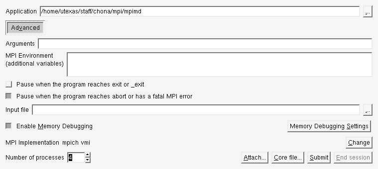
Session control window for DDT. This where you specify the executable path, command-line arguments and processor count.
(Clicking on the images will open them in a new window)
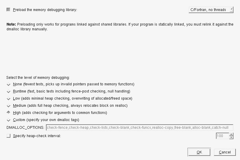
Different levels of memory debugging can be enabled. Since memory debugging is implemented using DMALLOC, you can customize using DMALLOC-supported options.
- DDT will thereafter submit a job to the development queue which will request the specified number of processors for 30 minutes. The DDT session will not start until the required resources are available for the debugging job. When the job starts running, you should see the following window appear:
For more information on how to perform parallel debugging using DDT, please consult the DDT user guide.
Click on Header to expand or collapse section. PDF of Optimization section
The most practical approach to enhance the performance of applications is to use use advanced compiler options, employ high performance libraries for common mathematical algorithms and scientific methods, and tune the code to take advantage of the architecture. Compiler options and libraries can provide a large benefit for a minimal amount of work. Always profile the entire application to ensure that the optimization efforts are focused on areas with the greatest return on the optimization efforts.
"Hot spots" and performance bottlenecks can be discovered with basic profiling tools like prof and gprof. It is important to watch the relative changes in performance among the routines when experimenting with compiler options. Sometimes it might be advantageous to break out routines and compile them separately with different options that have been used for the rest of the package. Also, review routines for "hand-coded" math algorithms that can be replaced by standard (optimized) library routines. You should also be familiar with general code tuning methods and restructure statements and code blocks so that the compiler can take advantage of the microarchitecture.
Code should:
- be clear and comprehensible
- provide flexible compiler support
- should be portability
Some best practices are:
- Avoid excessive program modularization (i.e. too many functions/subroutines)
- write routines that can be inlined
- use macros and parameters whenever possible
- Minimize the use of pointers
- Avoid casts or type conversions, implicit or explicit
- Avoid branches, function calls, and I/O inside loops
- structure loops to eliminate conditionals
- move loops around subroutine into the subroutine
Compiler options must be used to achieve optimal performance of any application. Generally, the highest impact can be achieved by selecting an appropriate optimization level, by targeting the architecture of the computer (CPU, cache, memory system), and by allowing for interprocedural analysis (inlining, etc.). There is no set of options that gives the highest speed-up for all applications and consequently different combinations have to be explored.
PGI compiler :
| -O[n] | Optimization level, n=0, 1, 2 or 3 |
| -tp barcelona-64 | Targeting the architecture |
| -Mipa[=option] | Interprocedural analysis, option=fast,inline |
Intel compiler :
| -O[n] | Optimization level, n=0, 1, 2 or 3 |
| -x[p] | Targeting the architecture, p=W or O |
| -ip, -ipo | Interprocedural analysis |
See the Development section for the use of these options.
TACC provides several ISP (Independent Software Providers) and HPC vendor math libraries that can be used in many applications. These libraries provide highly optimized math packages and functions for the Ranger system.
The ACML library (AMD Core Math Library) contains many common math functions and routines (linear algebra, transformations, transcendental, sorting, etc.) specifically optimized for the AMD Barcelona processor. The ACML library also supports multi-processor (threading) FFT and BLAS routines. The Intel MKL (Math Kernel Library) has a similar set of math packages. Also, the GotoBLAS libraries contain the fastest set of BLAS routine for this machine.
The default compiler representation for Ranger consists of 32-bit ints, and 64-bit longs and pointers.
Likewise for Fortran, integers are 32-bit, and the pointers are 64-bit.
This is called the LP64 mode (Long and Pointers are 64-bit, ints and integers are 32-bit).
Libraries with 64-bit integers are often suffixed with an IPL64.
ACML and MKL libraries
The "AMD Core Math Library" and "Math Kernel Library" consists of functions with Fortran, C, and C++ interfaces for the following computational areas:
- BLAS (vector-vector, matrix-vector, matrix-matrix operations) and extended BLAS for sparse computations
- LAPACK for linear algebraic equation solvers and eigensystem analysis
- Fast Fourier Transforms
- Transcendental Functions
Note, Intel provides performance libraries for most of the common math functions and routines (linear algebra, transformations, transcendental, sorting, etc.) for their em64t and Core-2 systems. These routines also work well on the AMD Opteron microarchitecture. In addition, MKL also offers a set of functions collectively known as VML -- the "Vector Math Library". VML is a set of vectorized transcendental functions which offer both high performance and excellent accuracy compared to the libm, for vectors longer than a few elements.
GotoBLAS library
The "GotoBLAS Library" (pronounced "goat-toe") contains highly optimized BLAS routines for the Barcelona microarchitecture. The library has been compiled for use with the PGI and Intel Fortran compilers on Ranger. The Goto BLAS routines are also supported on other architectures, and the source code is available free for academic use (download). We recommend the GotoBLAS libraries for performing the following linear algebra operations and solving matrix equations:
- BLAS (vector-vector, matrix-vector, matrix-matrix operations)
- LAPACK for linear algebraic equation solvers and eigensystem analysis
Additional performance can be obtained with these techniques :
- Memory Subsystem Tuning : Optimize access to the memory by minimizing the stride length and/or employ cache blocking techniques.
- Floating-Point Tuning : Unroll inner loops to hide FP latencies, and avoid costly operations like divisions and exponentiations.
- I/O Tuning : Use direct-access binary files to improve the I/O performance.
- Intel 64 Architecture
- Intel 10.1 Compilers
- Intel 9.1 C++ Compiler Documentation
- Intel 9.1 Fortran Compiler Documentation
- SSH Website
- TACC Introduction to SSH
- TACC Detailed Review of SSH
- "High Performance Computing" by Kevin Dowd and Charles Severance (O'Reilly book)